Analyze image stack of turbulent box
[1]:
import imageio

import matplotlib.pyplot as plt

import astro3d
from astro3d import image_stack
Read the image stack
We again need to set the printer-specific settings and the directory of the slides:
[2]:
stack = image_stack.IStack(
    astro3d.get_output('slices_turbulent_box'),
    dpi_x=600, dpi_y=300, dz=27e-4,
)
Print out statistics
[3]:
stack._get_colors(N=1)
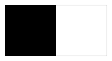
stack.show_colors()
getting colors from 1 sample images ... Done!
[3]:
(<Figure size 200x100 with 1 Axes>, <Axes:>)

Now we assign the transparent color index
[4]:
stack.empty_indices = [1]
[5]:
stack.show_info()
There are 2 colors in this image:
- [0, 0, 0]
- [255, 255, 255] (transp.)
185 files
dimension = 5.00 x 5.00 x 0.50 cm
filling fraction: 1.98%
nr of fully transparent columns: 0.35%
most opaque pixel has 97 filled pixels (=52.43% of all layers are filled)
mean counts in non-transparent columns: 10, 1.8e+02
Plots
Show the distribution of materials
[6]:
f, ax = stack.show_counts()

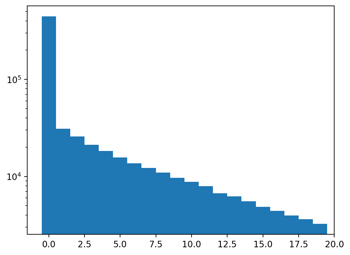
Show a histogram of the columns that are not fully transparent
[7]:
f, ax = stack.show_histogram()

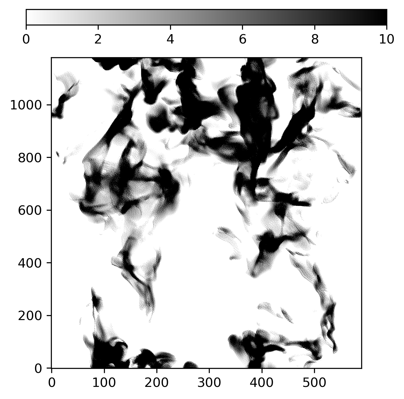
Show fully transparent pixels and the density distribution.
[8]:
f, ax = stack.show_transparency_estimate()

Top view
[9]:
img = stack.get_top_view(bg=[255, 255, 255]);
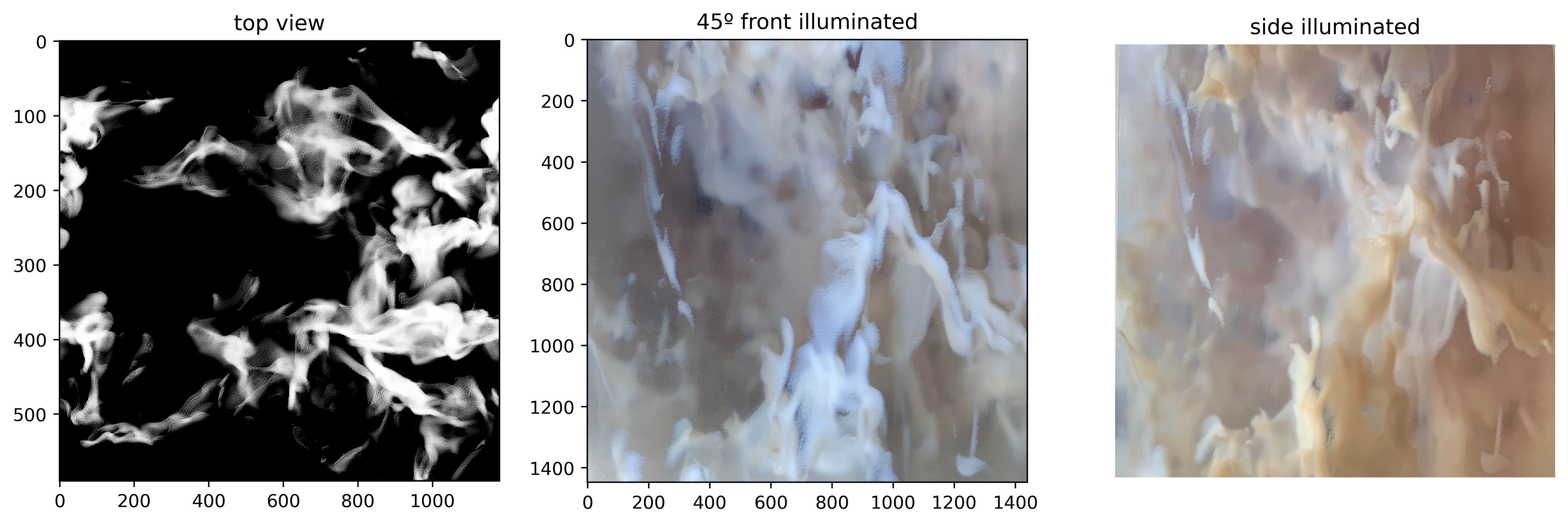
Compare data to 3d-printed result
[10]:
f, axs = plt.subplots(1, 3, dpi=200, figsize=(15,5))
axs[0].imshow((255 - img.transpose(1, 0, 2)) / 255.)
axs[0].set_aspect(stack.dpi_x / stack.dpi_y)
axs[0].set_title(f'top view')

axs[1].imshow(imageio.v2.imread('results/img1.jpg'))
axs[1].set_title('45º front illuminated')
axs[2].axis('off')

axs[2].imshow(imageio.v2.imread('results/img2.jpg'))
axs[2].set_title('side illuminated')
axs[2].axis('off');

[11]:
from IPython.display import Video
Video('results/turbulent_box.mp4', width=500, html_attributes='autoplay loop')
[11]: